Chapter 5 Cut Scores and Abnormality
Because that’s not what normal people do. — things my spouse says
You’ll recall that I previously warned against possible negative consequences of setting arbitrary cut points to dichotomize a data set—that is, turning numerical data on a continuous scale into two categories by using a cutoff value. But now consider the following scenarios:
To pass the written test for your a driving learner’s permit in California, you must answer at least 38 questions correctly out of 46. That’s 82.6% correct. At 80.4% (37/46) or below, you fail and have to retake the test on another day.
A patient’s blood test shows levels of ALT (alanine aminotransferase) at 77 units per liter. The lab report labels this as “abnormally” high, and the physician is concerned about possible liver damage or disease.
These two examples involve just the kind of dichotomization that I cautioned against, and yet they occur very commonly in practice. So what gives? Is it wrong to use cutoffs this way? Why do people do it?
The short answer is that we often find ourselves in need of a classification (pass or fail; diagnose liver disease or not) but without a perfect classification device. Rather we have only indirect measurements (of knowledge or liver function) in some quantitative measure. Perhaps you once found yourself on the “border” between letter grades for a course and were particularly perturbed (or relieved) by the imperfections of such a system. Or you may have found yourself with “slightly” abnormal levels in a blood test and wondered whether you should seek further tests.
Both the California department of motor vehicles and the physician in our scenarios need to make a decision based on imperfect evidence. They want to be able to say that the person’s test results show that they are ready to get behind the wheel of a car, in one scenario, or suffering from liver problems in the other. But all they can really do is express this belief using a probability. This probabilistic judgement is based on a mathematical model that relates traits like readiness-to-drive or liver-disease to certain test results. Understanding how these models come into existence is one of the learning objectives of this course.
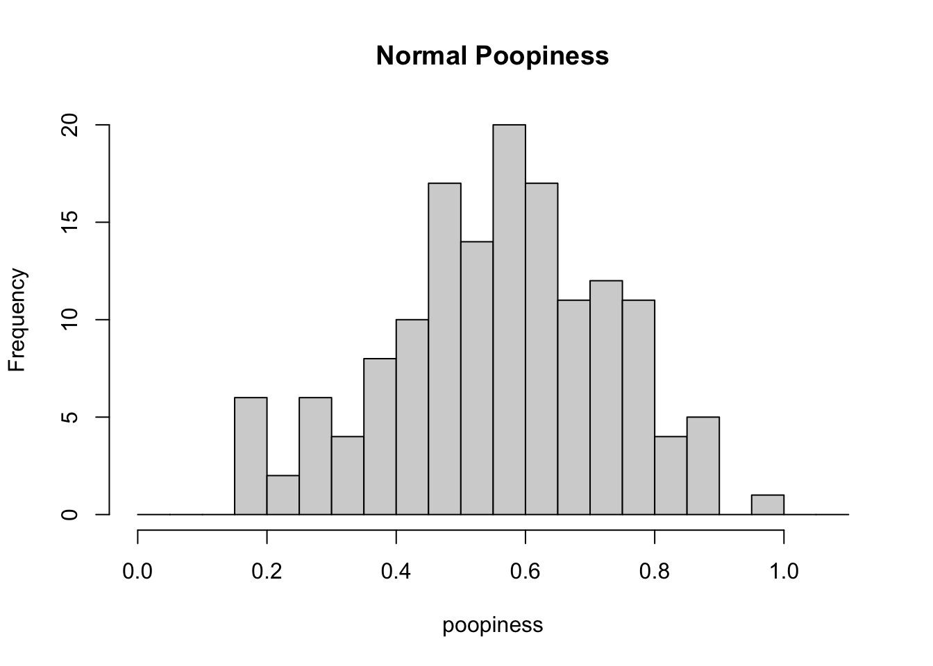
The term normal distribution arose in statistics because the particular bell-shaped distribution occurs so frequently. If poopiness were normally distributed in our sample from before it might look like this.

Figure 5.1: Normal poopiness
Technically speaking, all of the values, including the maximal value of 0.962 that we observe in Figure 5.1 are normal. Poopiness varies in the population. It is impossible to be abnormally poopy, under the circumstances. By definition, some values at the extreme ends of a normal distibution are less likely to occur than values in the middle. But still they may occur rarely. It is only when extreme values (large or small) are associated with other conditions of interest, such as the relationship between elevated ALT and liver disease, that it makes sense to “flag” these extreme values.
We say that we discretize continuous variables (i.e., turn them into discrete categorical variables) by using thresholds or cut scores. Passing a test or being flagged for liver disease is usually based on a single cut score. The cut score is a numerical value, and data that fall above or below that value are categorized differently. It is possible to use more than one threshold. For example, in the next chapter we will see that people can be classified as belonging to different generations based on their age, and neighborhoods can be categorized based on their population density.
We started out this course on a quest to answer our first big question: How many kinds of people are there? En route, we have examined both categorical data, such as from two-kinds-of-people questions, and numerical values like poopiness. The toilet paper and peanut butter orientation questions may seem silly and inconsequential to you. I can only imagine what you might think of the poopiness and crappiness dimensions that I completely made up (I admitted it!). However, in the next chapter we will see how some more standard variables are used to profile American people. Next week, we will see more issues of discrete/categorical and continous/numerical multi-dimensional descriptions of people that arise when it comes to personality psychology.